Animal experiments
All mice used in this study were Cast-EiJ/Bl6 mice and were bred and maintained in the Hubrecht Institute Animal Facility. All mouse experimentation was approved by the Animal Experimentation Committee (DEC) from the Koninklijke Nederlandse Akademie van Wetenschappen (KNAW) and complied with existing European Union legislation and local standards.
Mouse bone marrow
Male 13-week-old C57BL/6 mice were used to extract bone marrow cells. Femurs and tibia were extracted, the bone ends were cut away to access the bone marrow, which was flushed out using a 22G syringe with HBSS (– calcium, – magnesium, – phenol red, Gibco, catalog no. 14175053) supplemented with Pen-Strep and 1% fetal calf serum. The bone marrow was dissociated and debris removed by passing through a 70 μm cell strainer (Corning, catalog no. 431751). Cells were washed with 25 ml supplemented HBSS before depleting the sample of unnucleated cells using IOTest 3 Lysing solution (Beckman Coulter) following the providerʼs instructions. Cells were washed an additional two times with PBS before processing them by the sortChIC protocol for histone modifications. For whole bone marrow experiments (that is, not enriched for specific cell types), we processed cells using the sortChIC protocol for unfixed cells (without ethanol fixation). For the ground truth experiment with sorted cell types, we processed cells using the sortChIC protocol for ethanol-fixed cells. For ethanol fixation, cells were resuspended in 70% ethanol and fixed for 1 h at –20 °C. Afterwards cells were resuspended in Storage buffer (42.5 ml H2O RNAse free, 1 ml 1 M HEPES pH 7.5 (Invitrogen), 1.5 ml 5 M NaCl, 3.6 μl spermidine (Sigma Aldrich, catalog no. S2626-5G), protease inhibitor (Sigma Aldrich, catalog no. 5056489001), 200 μl 0.5 M EDTA, 5 μl dimethylsulfoxide) and frozen at –80∘C, before processing by the sortChIC protocol.
Mouse organogenesis
No randomization or blinding was performed. Sex of embryos was not known at the time of collection. Four to five embryos were pooled for each reported timepoint (E9.5, E10.5, E11.5) before single-cell isolation. Pooled embryos were dissociated in TrypleE for 10 min at room temperature. Undigested portions were physically removed and the remainder filtered through a 30 μm filter before the single-cell suspension was split into three samples for each timepoint and each scChIX-seq experiment. Per timepoint, two single-cell samples were used each for a single antibody incubation (H3K36me3 or H3K9me3) and one sample for the double antibody incubation (H3K36me3 + H3K9me3). Antibody incubation was performed as described in the scChIX-seq protocol before single-cell capture using flow cytometry. A DNA library was prepared for each sample using the sortChIC protocol for unfixed cells.
In vitro macrophage differentiation
For in vitro differentiation of bone marrow-derived macrophages, bone marrow was collected aseptically by flushing tibia and femurs from euthanized wild-type male C57BL/6 mice with sterile RPMI and 10% FCS through a 70 μm cell strainer (Corning). To enrich for stem and progenitor cells, lineage marker-positive (Lin+) cells were depleted by magnetic-activated cell sorting using a mouse Lineage Cell Depletion kit (Miltenyi Biotec). Lin– cells were cultured on nontissue-culture-treated plates (Corning) for 7 days in RPMI medium supplemented with 10% FCS, 100 IU ml–1 penicillin, 100 mg ml–1 streptomycin and 10 ng ml–1 recombinant murine MCSF (Peprotech). Medium was refreshed after 3 days. Every 24 h, suspension cells were collected and adherent cells were harvested by incubating 10 min in 2 mM EDTA/0.5% BSA in PBS. Suspension and adherent cells were combined and stained with CellTrace fluorescent labels (Thermo Fisher), according to manufacturer’s instructions. Briefly, cells were pelleted and resuspended in 37 °C PBS containing fluorescent dyes (working concentrations CellTrace CSFE (CTC): 2.5 μM; CellTrace Yellow (CTY): 2.5 μM; CellTrace Far Red (CTFR): 0.5 μM) at a concentration of 1,000,000 cells ml–1. Cells were incubated at 37 °C protected from light for 20 min. Staining reactions were stopped by adding two volumes of RPMI/10% FCS and incubating for 5 min at room temperature, protected from light, after which cells were washed twice in PBS. The following combinations of labels were used: unstained (day 0), CTC (day 1), CTY (day 2), CTFR (day 3), CTC + CTY (day 4), CTC + CTFR (day 5), CTY + CTFR (day 6) and CTC + CTY + CTFR (day 7). After harvesting and staining, cells were fixed in 70% ethanol for 1 h and stored for later by the sortChIC protocol for fixed cells.
Cell preparation without ethanol fixation for sortChIC experiments
Cells from whole bone marrow (H3K4me1+H3K27me3) and mouse embryos (H3K36me3+H3K9me3) were processed using the sortChIC method without ethanol fixation. Cells were processed in 0.5 ml protein low-binding tubes. Following steps were performed on ice. Cells were resuspended in 500 μl wash buffer (47.5 ml H2O RNAse free, 1 ml 1 M HEPES pH 7.5 (Invitrogen), 1.5 ml 5M NaCl, 3.6 μl pure spermidine solution (Sigma Aldrich)). Cells were pelleted at 600g for 3 min and resuspended in 400 μl wash buffer 1 (wash buffer with 0.05% saponin (Sigma Aldrich), protease inhibitor cocktail (Sigma Aldrich), 4 μl 0.5 M EDTA) containing the primary antibody (1:100 dilution for the antibody, saponin has to be prepared fresh every time as a 10% solution in PBS). Cells were incubated overnight at 4 °C on a roller, before being washed once with 500 μl wash buffer 2 (wash buffer with 0.05% saponin, protease inhibitor). Afterwards cells were resuspended in 500 μl wash buffer 2 containing Protein A-Micrococcal Nuclease (pA-MNase) (3 ng ml–1) and incubated for 1 h at 4 °C on a roller.
Finally, cells were washed an additional two times with 500 μl wash buffer 2 before passing it through a 70 μm cell strainer (Corning, catalog no. 431751) and sorting G1 cells based on Hoechst staining on a BD Influx FACS machine into 384-well plates containing 50 nl wash buffer 3 (wash buffer containing 0.05% saponin) and 5 μl sterile filtered mineral oil (Sigma Aldrich) per well. Small volumes were distributed using a Nanodrop II system (Innovadyme).
Cell preparation with ethanol fixation and surface antibody incubation for sortChIC experiments
Cells from sorted bone marrow (H3K27me3+H3K9me3) and macrophage in vitro differentiation (H3K4me1+H3K36me3) were processed using the ethanol fixation protocol. Sorted bone marrow cells were also incubated with surface antibody to enrich for known cell types. For the ethanol-fixed cells the above described sortChIC protocol was adapted. Wash buffers were used as described above, except that 0.05% saponin was exchanged for 0.05% Tween. Ethanol-fixed cells were thawed on ice. Cells were spun at 400g for 5 min and washed once with 400 μl wash buffer 1. Cells were spun again at 400g and resuspended in 400 μl wash buffer 1. Cell suspension was split into three samples each having a volume of 400 μl and incubated with one or two antibodies (1:100 dilution for the antibody) overnight on a roller at 4 °C. The next day, cells were spun at 400g, washed once with 400 μl wash buffer 2 and resuspended in 500 μl wash buffer 2 containing pA-MNase (3 ng ml–1) and incubated for 1 h on a rotator at 4 °C. Next, cells were spun at 400g and resuspended in 400 μl wash buffer 2 (with addition of 5% blocking rat serum). To sort for defined cell types in the ground truth bone marrow experiment, surface antibodies were added according to these concentrations and were incubated for 30 min on ice:
$$begin{array}{l}begin{array}{ll}{{mbox{antibody}}},&,{{mbox{info}}}\ {{mbox{GR1}}},&,{{mbox{A647, anti-mouse Ly-6G/Ly-6C (Gr-1) Antibody,}}}\ & {mbox{clone: RB6-8C5}}\ {{mbox{NK1}}},&,{{mbox{A488, anti-mouse NK-1.1 Antibody, clone: PK136}}}\ {{mbox{CD19}}},&,{{mbox{BV421, anti-mouse CD19 Antibody, clone: 6D5}}}end{array}\begin{array}{l}{{mbox{working concentration}}}\1:8,000\1:400\1:200end{array}end{array}$$
BD FAC software v.1.2.0.142 was used to collect data from the FACS machine during cell sorting; see Supplemental Fig. 1 for the gating strategy.
Finally, samples were washed once with 500 μl wash buffer 2 before passing them through a 70 μm cell strainer (Corning, catalog no. 431751) and sorting on a BD Influx FACS machine, with surface antibody specific gating, into 384-well plates containing 50 nl wash buffer 3 (wash buffer containing 0.05% Tween) and 5 μl sterile filtered mineral oil (Sigma Aldrich) per well. Small volumes were distributed using a Nanodrop II system (Innovadyme).
MNase activation for sortChIC experiments
Targeted fragmentation was started by the addition of 5 μl wash buffer 2 containing 4 mM CaCl2. For digestion, plates were incubated for 30 min in a PCR machine set at 4 °C. Afterwards the reaction was stopped by adding 100 nl of a stop solution containing 40 mM EGTA, 1.5% NP40, and 10 nl 2 mg ml−1 proteinase K. Plates were incubated in a PCR machine for further 20 min at 4 °C, before chromatin was released and pA-MNase permanently destroyed by proteinase K digestion at 65 °C for 6 h followed by 80 °C for 20 min to heat inactivate proteinase K. Afterwards plates were stored at –80 °C until further processing.
Library preparation for sortChIC experiments
DNA fragments were blunt ended by adding 150 nl end repair mix per well and incubating for 30 min at 37 °C followed by 20 min at 75 °C for enzyme inactivation. End repair mix per well: Klenow large (NEB, catalog no. M0210L) 2.5 nl, T4 PNK (NEB, catalog no. M0201L) 2.5 nl, dNTPs 10 mM 6 nl, ATP 100 mM 3.5 nl, MgCl2 25 mM 10 nl, PEG8000 50% 7.5 nl, PNK buffer 10× (NEB, catalog no. B0201S) 35 nl, BSA 20 ng 1.8 nl, nuclease-free water 81.3 nl.
Blunt fragments were subsequently A-tailed by adding 150 nl per well of A-tailing mix and incubated for 15 min at 72 °C. Through the strong preference of AmpliTaq 360 to incorporate dATP as a single base overhang even in the presence of other nucleotides, a general dNTP removal was not necessary. A-tailing mix per well: AmpliTaq 360 (Thermo Fisher Scientific, catalog no. 4398828) 1 nl, dATPs 100 mM 1 nl, KCl 1 M 25 nl, PEG8000 50% 7.5 nl, BSA 20 ng 0.8 nl, nuclease-free water 114.8 nl.
Fragments were ligated to T-tail containing forked adapters containing a T7 polymerase binding site for in vitro transcription (IVT)-based amplification.
Top strand: 5′-GGTGATGCCGGTAATACGACTCACTATAGGGAGTTCTACAGTCCGACGATCNNNACACACTAT-3′
Bottom strand: 5′-TAGTGTGTNNNGATCGTCGGACTGTAGAACTCCCTATAGTGAGTCGTATTACCGGCGAGCTT-3′
The three random nucleotides (NNN) were the unique molecular identifier used for read deduplication and the eight bases afterwards represent the cell barcodes, which were different for each of the 384 wells. For a full list of adapters and the cell barcodes for each well, see the excel sheet in Supplemental Table 1. Cell barcodes for each 384-well plates are also found as a text file in the scChIX-seq Github repository: (https://github.com/jakeyeung/scChIX/blob/main/inst/extdata/cellbarcodes_384_NLA_annotated.bc).
For ligation, 50 nl of 5 μM adapter in 50 mM Tris pH 7 was added to each well with a Mosquito HTS (ttp labtech). After centrifugation, 150 nl of ligation mix was added before incubating plates for 20 min at 4 °C, followed by 16 h at 16 °C for ligation and 10 min at 65 °C to inactivate ligase. Adapter ligation mix per well: T4 ligase (400,000 U ml–1, NEB, catalog no. M0202L) 25 nl, MgCl2 1 M 3.5 nl, Tris 1 M pH 7.5 10.5 nl, DTT 0.1 M 52.5 nl, ATP 100 mM 3.5 nl, PEG8000 50% 10 nl, BSA 20 ng 1 nl, nuclease-free water 44 nl.
Before pooling, 1 μl nuclease-free water was added to each well to minimize material loss. Ligation products were pooled by centrifugation into oil coated VBLOK200 Reservoir (ClickBio) at 500g for 2 min and the liquid face was transferred into 1.5 ml Eppendorf tubes and then purified by centrifugation at 13,000g for 1 min and transferred into a fresh tube twice. DNA fragments were purified using Ampure XP beads (Beckman Coulter, prediluted one in eight in bead binding buffer: 1 M NaCl, 20% PEG8000, 20 mM Tris pH 8, 1 mM EDTA) at a bead to sample ratio of 0.8. After 15 min incubation at room temperature, beads were washed twice with 1 ml 80% ethanol resuspending the beads during the first wash and resuspended in 20 μl nuclease-free water. After 2 min elution, the supernatant was transferred into a fresh 0.5 ml tube. A second cleanup was performed adding 26 μl undiluted Ampure XP beads and the beads were resuspended in 8 μl nuclease-free water. The cleaned DNA was then linear amplified by IVT by adding 12 μl of MEGAscript T7 Transcription Kit (Fisher Scientific, catalog no. AMB13345) for 12 h at 37 °C. Template DNA was removed by addition of 2 μl–1 TurboDNAse (IVT kit) and incubation for 15 min at 37 °C. The RNA produced was further purified using RNA Clean XP beads (Beckman Coulter) at a beads to sample ratio of 0.8 and samples were resuspended in 22 μl of nuclease-free water. RNA was fragmented by mixing in 4.4 μl fragmentation buffer (200 mM Tris-acetate pH 8.1, 500 mM KOAc, 150 mM MgOAc) and incubation for 2 min at 94 °C. Fragmentation was stopped by transferring samples to ice, adding 2.64 μl 0.5 M EDTA and another bead cleanup; samples were resuspended in 12 μl nuclease-free water.
RNA (5 μl) was primed for reverse transcription by adding 0.5 μl 10 mM dNTPs and 1 μl 20 mM randomhexamerRT primer (5′-GCCTTGGCACCCGAGAATTCCANNNNNN-3′) and hybridizing it by incubation at 65 °C for 5 min followed by direct cool down on ice. Reverse transcription was performed by further addition of 2 μl first strand buffer (part of Invitrogen kit, catalog no. 18064014), 1 μl 0.1 M DTT, 0.5 μl RNAseOUT (Invitrogen, catalog no. LS10777019) and 0.5 μl SuperscriptII (Invitrogen, catalog no. 18064014) and incubating the mixture at 25 °C for 10 min followed by 1 h at 42 °C. Single-stranded DNA was purified through incubation with 0.5 μl RNAseA (Thermo Fisher, catalog no. EN0531) and incubation for 30 min at 37 °C.
A final PCR amplification to add the Illumina small RNA barcodes and handles was performed by adding 25 μl of NEBNext Ultra II Q5 Master Mix (NEB, catalog no. M0492L), 11 μl nuclease-free water and 2 μl of 10 μM RP1 and RPIx primers.
PCR protocol for sortChIC experiments
Activation for 30 s at 98 °C, 8–12 cycles (depending on starting material), 10 s at 98 °C, 30 s at 60 °C, 30 s at 72 °C, final amplification 10 min at 72 °C.
PCR products were cleaned by two consecutive DNA bead clean-ups with a bead to sample ratio of 0.8. Final product was eluted in 7 μl nuclease-free water. The abundance and quality of the final library were assessed by QUBIT and bioanalyzer.
Data processing
All DNA libraries were sequenced on a Illumina NextSeq500 with 2 × 75 bp. We ran the raw fastq files through the Single-Cell MultiOmics (SCMO) workflow (github.com/BuysDB/SingleCellMultiOmics52). The workflow comprises of six steps.
(1) Demultiplex raw fastq files using demux.py (SCMO). (2) Trim fastq files by removing adapters using cutadapt (v.3.5). (3) Map trimmed fastq files using bwa (v.0.7.17-r1188). (4) Tag bam files with cell barcode information, using bamtagmultiome.py (SCMO). (5) Generate count tables using bamToCountTable.py (SCMO). (6) Run dimensionality reduction of count matrices using run_LDA_model.R. See an example of the pipeline in the scChIX-seq Github repository53.
Unmixing scChIX-seq signal
Single-cell epigenomics techniques (for example, sortChIC, CUT&RUN and CUT&TAG) generate a vector of counts indicating the number of cut fragments that map in each genomic region for each cell. We model the vector of counts from a double-incubated cell (overrightarrow{y}) as a linear combination of two multinomial distributions: one coming from a cluster c of histone modification 1, parameterized by ({overrightarrow{p}}_{c}), the other from another cluster d of histone modification 2 ({overrightarrow{q}}_{d}). The log-likelihood for a linear combination of two multinomials is:
$${{{{rm{L}}}}}_{(c,d)}=log (Pleft(overrightarrow{y}| {overrightarrow{p}}_{c},{overrightarrow{q}}_{d},wright))propto mathop{sum }limits_{g=1}^{G}{y}_{g}log left(w{p}_{c,g}+left(1-wright){q}_{d,g}right).$$
(1)
(overrightarrow{y}) is the number of cuts across the genome for a double-incubated cell. pc,g and qd,g are cluster-specific probabilities indicating the likelihood that a cut fragment maps to region g in histone modifications 1 and 2, respectively. w is the mixing fraction of histone modification 1 in the double-incubated cell, which we estimate by maximizing the log-likelihood given (overrightarrow{y}), ({overrightarrow{p}}_{c}) and ({overrightarrow{q}}_{d}).
Applying single-cell techniques to complex tissues generates data with many clusters. Therefore, given a double-incubated cell, we do not know which pair of clusters (c,d) were combined to generate the observed counts. We therefore calculate the log-likelihood for all possible pairs of clusters learned from the training data and then select the cluster pair with the highest probability for each cell.
Cluster-specific probabilities ({overrightarrow{p}}_{c}) and ({overrightarrow{q}}_{d}) are learned by applying LDA (with k = 30 topics) using the topicmodels R package54 to the training data (that is, single-incubated cells), which are count matrices.
After assigning each cell to the most probable cluster pair ((hat{c},hat{d})), we assign yi,j, the jth read mapped to region g in cell i, to histone mark 1 with probability Pi,j:
$${P}_{mathrm{i,j}}=frac{w{p}_{hat{c},g}}{w{p}_{hat{c},g}+left(1-wright){q}_{hat{d},g}}.$$
(2)
This assignment generates a pair of vectors ({overrightarrow{y}}_{1,i}) and ({overrightarrow{y}}_{2,i}) that are linked because they both come from cell i. Unmixed counts ({overrightarrow{y}}_{1,i}) and ({overrightarrow{y}}_{2,i}) are then projected back onto the space inferred from training data of histone modification 1 and 2, respectively. The links between histone modification 1 and 2 are used to transfer labels and create linked UMAPs between the two histone modifications.
Latent Dirichlet allocation
LDA is a probabilistic matrix decomposition model that is useful when the input data is a matrix of counts. LDA uses hierarchical multinomial models to estimate the relative frequencies of cuts in each genomic region in single cells.
To generate the genomic location of the jth read for cell i:
Choose a topic zi,j by sampling from the cell-specific distribution of topics:
$$begin{array}{r}{overrightarrow{U}}_{mathrm{i}} sim ,{{{rm{Dirichlet}}}},(alpha )\ {z}_{mathrm{i,j}} sim ,{{{rm{Multinomial}}}},({overrightarrow{U}}_{i},1)end{array}$$
Choose genomic region wi,j by sampling from the topic-specific distribution of genomic regions:
$$begin{array}{r}{overrightarrow{V}}_{mathrm{k}} sim ,{{{rm{Dirichlet}}}},(delta )\ {w}_{mathrm{i,j}} sim ,{{{rm{Multinomial}}}},({overrightarrow{V}}_{{z}_{mathrm{i,j}}},1)end{array}$$
The Dirichlet distributions are priors to prevent overfitting when there are few cuts in the region. We used the LDA model implemented by the topicmodels R package, using the Gibbs sampling implementation with hyperparameters α = 1.67, δ = 0.1, where K is the number of topics23.
We estimate ({overrightarrow{p}}_{c}) and ({overrightarrow{q}}_{d}) for each cluster in histone modification 1 ({{overrightarrow{p}}_{1},{overrightarrow{p}}_{2},…,{overrightarrow{p}}_{C}}) and modification 2 ({{overrightarrow{q}}_{1},{overrightarrow{q}}_{2},…,{overrightarrow{q}}_{D}}) by averaging the estimated probabilities across cells assigned to each cluster for each gene g:
$$p_{g,c}=frac{1}{vert C vert}mathop{sum }limits_{mathrm{i}in C}mathop{sum }limits_{mathrm{k}=1}^{K}{V}_{mathrm{g,k}}{U}_{mathrm{k,i}}$$
where C is the set of cells that belong to cluster c.
Simulation of single- and double-incubated histone modification data
To simulate multimodal single-cell histone modification data with varying degrees of overlap, we extended simATAC55 to allow generating cell-type profiles from histone modifications of varying mutually exclusive relationships.
For each cell type, we first run simATAC to generate sparse count data of 10,000 loci across 750 cells partitioned into three technical replicates of 250 cells each. The high-dimensional count data are sparse. Counts from each locus are generated according to a Poisson likelihood with locus-specific means (λ) matching real single-cell ATAC-seq from K562 cells (GSE99172).
In our 750 cells, cells 1–250 represent single-incubated cells from mark 1; cells 251–500 from mark 2; cells 501–750 from double-incubated cells. Cells from mark 1 have counts generated from locus-specific means λ. Cells from mark 2 also have counts generated from λ, but we swap the top x% of bins with highest λ with bins with lowest λ, allowing precisely defined sets of mutually exclusive and overlapping bins. We use x = 1%, 50% and 99% to benchmark our method from mostly overlapping (that is x = 1%) to mostly mutually exclusive (that is x = 99%) Cells from mark 3 are generated by adding counts generated from mark 1 and mark 2 to simulate double-incubated cells.
To generate cell-type-specific profiles, we repeat the above with a cell-type-specific random seed and shuffle the order of the bins. This generates count data where λ is cell-type specific, but the distribution of λ are preserved genome-wide.
Estimating the top cluster-specific bins
We use the LDA matrix factorization to identify the top cluster-specific bins in the data. We rank the bin loadings for each cell type and take the top 150 (whole bone marrow) or 250 (mouse organogenesis) bins with the largest loadings.
Inferring pseudotime in differentiation data
To analyze the macrophage differentiation data, we first removed erythroblasts, plasmacytoid dendritic cells, and innate lymphocyte cells from the data, which were concentrated at day 0 and not considered to be part of the macrophage differentiation trajectory. We then ran LDA (k = 30 topics) and performed principal component analysis (PCA) on the LDA outputs, which retrieves the principal components that explain the largest amount of variance after denoising the data. We used the first principal component for H3K4me1 and H3K36me3 to define pseudotime, which we found correlates with the day along the timecourse.
Unmixing scChIX-seq signal from continuous pseudotime
To apply scChIX-seq on continuous pseudotime, we modify the log-likelihood (equation (1)) to account for a continuous variable:
$${{{rm{L}}}}left({t}_{1},{t}_{2}right)=log left(Pleft(overrightarrow{y}| overrightarrow{p}left({t}_{1}right),overrightarrow{q}left({t}_{2}right),wright)right)propto mathop{sum }limits_{g=1}^{G}{y}_{g}log left(w{p}_{g}left({t}_{1}right)+left(1-wright){q}_{g}left({t}_{2}right)right)$$
(3)
where t1 ∈ [0, 1] is pseudotime from histone modification 1 and t2 ∈ [0, 1] is pseudotime from modification 2.
To estimate pseudotime, we ran LDA to denoise the count matrix, and then ran PCA to estimate largest principal components explaining the variance in the data. We took the first principal component as our pseudotime estimate for both marks, which captured the epigenomic changes over the 7-day timecourse.
({p}_{g}left(tright)) is estimated by fitting the signal from histone modification 1 at genomic region g with a lowess curve along pseudotime. We estimate qg analogously but using signal from histone modification 2.
To infer the pseudotime of histone modifications 1 and 2 simultaneously given a vector of counts from a double-incubated cell, we estimate t1 and t2 that minimizes the log-likelihood L from equation (3). We estimate the variance-covariance matrix of t1 and t2 by the square root of the inverse of the Hessian matrix, which we use to calculate the standard errors.
Since the t1 and t2 are constrained between 0 and 1, we use the L-BFGS-B optimization algorithm implemented in R. Since estimates from a single cell can sometimes be noisy due to low counts, we sum the counts across the 25-nearest neighbors (estimated from the latent space inferred by LDA) for each double-incubated cell.
Chromatin velocity during macrophage differentiation
We assume that dynamic genomic regions in H3K36me3 can be modeled using a first-order differential equation
$$frac{d{K}_{36}left(tright)}{dt}={K}_{4}left(tright)-gamma {K}_{36}left(tright).$$
(4)
We estimate the time constant γ for each genomic region by fitting an exponential relaxation function across pseudotime
$${K}_{36}left(tright)={y}_{0}+Aleft(1-{e}^{-gamma t}right),$$
(5)
where y0 is the signal at t = 0 and A is the predicted H3K36me3 levels at steady state. Fitting the γ directly from the pseudotime allows us to leverage signal from both single- and deconvolved cells.
To predict future values of H3K36me3 levels for each cell at each genomic region, we use the Euler method and plug in the estimated γ, H3K4me1 levels at time t and time step h of 0.02 pseudotime units:
$${K}_{36}left(t+1right)={K}_{36}left(tright)+hleft({K}_{4}left(tright)-gamma {K}_{36}left(tright)right).$$
(6)
Finally, we project the single- and double-incubated H3K36me3 signal onto the first two principal components and project the predicted future values onto the PCA. We use the velocity grid flow visualization as implemented in velocyto56 to visualize the velocity vectors on the PCA space.
Comparison with multi-CUT&TAG
Raw fastq files (R1, R2 and R3) from the single-cell experiments were downloaded from Gene Expression Omnibus accession number GSE171554. The first 42 bases of the reads in R1 and R2 were trimmed to remove the barcodes and the bases common to all Tn5 adapter sequences. The 16-base cell barcodes in R3 were added to the fastq headers of R1 and R2. The trimmed and cell-barcoded R1 and R2 reads were then aligned to the mm10 mouse genome using Burrows-Wheeler aligner (bwa v.0.7.17-r1188). Fragments that start at same location and have the same cell barcode were considered duplicates and discarded. Cells with more than 100 fragments with MAPQ scores in R1 greater than or equal to 40 were kept for comparison with scChIX-seq.
Reporting summary
Further information on research design is available in the Nature Portfolio Reporting Summary linked to this article.